컴퓨터 비전 책을 통해서 배운 SIFT 특징점 검출 알고리즘을 python으로 직접 구현 해봅시다.
SIFT에 대한 개념은 위키백과에 자세히 설명돼 있습니다.
https://en.wikipedia.org/wiki/Scale-invariant_feature_transform
Scale-invariant feature transform - Wikipedia
From Wikipedia, the free encyclopedia Feature detection algorithm in computer vision The scale-invariant feature transform (SIFT) is a computer vision algorithm to detect, describe, and match local features in images, invented by David Lowe in 1999.[1] App
en.wikipedia.org
코드의 자세한 내용은 주석을 확인해 주세요.
Code
import cv2
from matplotlib.style import library
import numpy as np
import math
from matplotlib import pyplot as plt

def G_filter(k, sigma, v):

    assert k % 2 == 1, 'kernel_size must be odd' # filter must be odd_size

    n = int((k - 1) / 2) # number to get range of filter
    l = []

    for i in range(-1 * n, n + 1):
        for j in range(-1 * n, n + 1):
            c = -1 * ( ( i**2 + j**2 ) / (2 * sigma**2) )
            # definition of Gaussian filter
            l.append(c)

    gaussian = np.exp(l).reshape(-1, k) # take exponential
    sum = gaussian.sum() # normalization factor

    if v == 1:
        return gaussian / sum # version #1
    if v == 2:
        return gaussian # version #2

def padding(img, n):

    x, y = img.shape # original image size

    padding_img = np.zeros((x+2*n, y+2*n)) # consider up,down,left,right

    padding_img[n:x+n, n:y+n] = img # zero padding

    return padding_img

def conv(img, filter):

    k = len(filter) # kernel size
    n = int((k - 1) / 2) # padding number
    x, y = img.shape # original image size

    a = padding(img, n)

    for i in range(n, x+n):
        for j in range(n, y+n):
            a[i][j] = np.multiply(a[i-n:i+n+1, j-n:j+n+1], filter).sum() # convolution operation

    return a[n:x+n, n:y+n] # return result image ,except the padding part

def sift(img, G, d_G, k, count):
    # src, Gaussian list, DOG list, k is number of octave, count is now octave

    G[count].append(img)
    sigma = 1.6 # first 1.6

    for i in range(5):
        sigma = math.sqrt( (2 ** (2/3)) - 1 ) * sigma # difference between images in octave
        filter = G_filter(3, sigma, 1)
        img = conv(img, filter)
        G[count].append(img)
        d_G[count].append(G[count][i+1] - G[count][i]) # DOG

    if count < k-1: # recursive call
        img = G[count][3] # sigma is 3.2
        img = img[0::2,0::2] # downsampling 2
        count += 1

        sift(img, G, d_G, k, count)


def finding_key(d_G, key_points, k, count):
    m, n = d_G[count][0].shape # now octave's size
    key_thr = [33, 1, 0.1, 0.01, 0.001]

    for z in range(1,4): # because first and last DOG not used
        for i in range(1, int((m / (2 ** count)) -1)):
            for j in range(1, int( (n / (2 ** count)) -1 )): # except frame

                lower_dog = d_G[count][z-1][i-1:i+2, j-1:j+2] # down
                lower_dog = lower_dog / lower_dog.sum() # normalization

                now_dog = d_G[count][z][i-1:i+2, j-1:j+2] # now
                now_dog = now_dog / now_dog.sum()

                upper_dog = d_G[count][z+1][i-1:i+2, j-1:j+2] # up
                upper_dog = upper_dog / upper_dog.sum()
                if lower_dog.size == 0:
                    continue
                space = np.vstack((upper_dog, now_dog, lower_dog)).reshape(3,3,3)
                # finding space to get key points

                if now_dog[1][1] == space.min() or now_dog[1][1] == space.max():
                    # print(count , now_dog[1][1])
                    # search now_dog center whether local minimum or maximum
                    if now_dog[1][1] > key_thr[count] or now_dog[1][1] < -1 * key_thr[count]: # not noise
                        i = i * 2**(count)
                        j = j * 2**(count) # scaling size to original image

                        key_points.append((i, j, z, count)) # count is which octave is

    if count < k-1:
        count += 1
        finding_key(d_G, key_points, k, count) # recursive
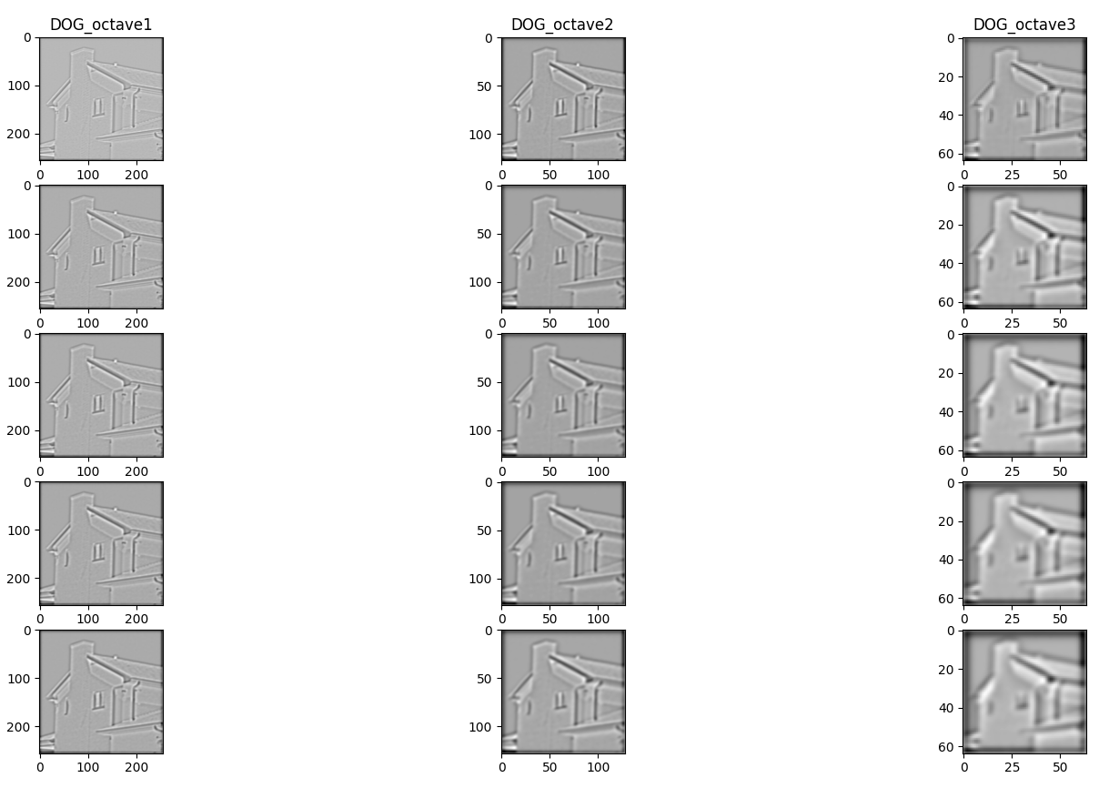
가장 중요한 DOG( difference of Gaussian )을 구하기만 하면 준비과정은 끝나고 이후 finding_key() 함수의 알고리즘을 통해 키포인트를 찾아냅니다.
Gaussian Space

DOG
이제 키포인트 알고리즘에 따라 찾은 키포인트에 원을 그려 보고 opencv에서 제공하는 라이브러리와 비교해봅시다
참고로 라이브러리 사용방법은 아래와 같습니다.
Code
import cv2
from matplotlib import pyplot as plt

imageFile = '../house.bmp'
img1 = cv2.imread(imageFile, 0)

# SIFT 추출기 생성
sift = cv2.SIFT_create()
# 키 포인트 검출과 서술자 계산
keypoints, descriptor = sift.detectAndCompute(img1, None)
print('keypoint:',len(keypoints), 'descriptor:', descriptor.shape)
print(descriptor)

# 키 포인트 그리기
img_draw = cv2.drawKeypoints(img1, keypoints, None, \
                flags=cv2.DRAW_MATCHES_FLAGS_DRAW_RICH_KEYPOINTS)
# 결과 출력
plt.imshow(img_draw, cmap='gray')
plt.title('key')
plt.show()
 |
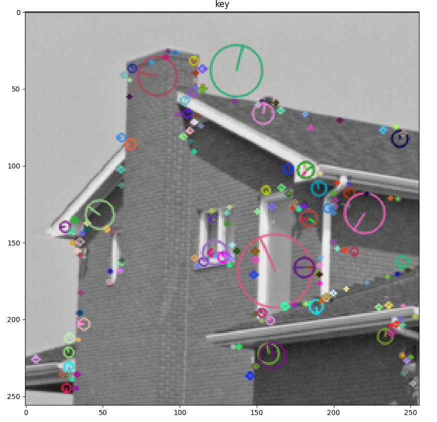 |
| 직접 구현한 SIFT | opencv 라이브러리 사용 |
분석
키포인트의 정확도나 개수등에서 라이브러리랑 큰 차이를 보였습니다. 실제로 opencv는 특징점(코너, 엣지)이 되는 부분을 정확히 찾은 반면 직접 구현한 SIFT는 특징점을 찾은것 같으나 다소 영점이 안맞고 조금 떨어진 부분을 찾았습니다. 논문에서는 테일러 급수를 사용해서 좌표를 조정했다고 되어있으나 그 자세한 과정은 직접 구현할때 생략했기 때문에 이러한 결과가 나왔다고 생각합니다. 하지만 논문과 책을 읽고 알고리즘을 이해한 상태에서 직접 구현을 해볼수도 있다는 생각이 들었고 아직 부족하지만 개선해 나가면서 배울부분도 많다고 생각합니다.
감사합니다.
'컴퓨터 비전 > 실습' 카테고리의 다른 글
| prewitt, sobel, canny 구현(python) (0) | 2023.02.10 |
|---|---|
| mean shift 직접 구현하기(python) (0) | 2023.01.31 |
| kmeans 직접 구현하기(python) (1) | 2023.01.25 |
| Bilateral Filter 직접 구현하기(python) (0) | 2023.01.18 |


