Mean Shift
이번 포스팅에서는 mean shift 알고리즘을 직접 구현해보도록 하겠습니다.
산 정상을 가장 빨리 도착하는 방법은 등고선 지도에서 선이 조밀한 곳을 직선거리로 가는 방법일 것입니다.
이처럼 어떤 값의 분포중심을 찾는 방법이 mean shift (평균 이동) 알고리즘 입니다.
구현방법은 데이터 중심으로부터 반경 R안에 있는 전체 데이터의 무게중심을 구하고 중심을 무게중심으로 이동시켜 다시 그 과정을 수렴할때까지 반복하면 됩니다. 따라서 k means 알고리즘과 달리 사람이 직접 k개로 데이터를 나누지 않아도 적절히 세그멘테이션이 가능합니다. 하지만 모든 데이터에 대해 수렴점을 찾기때문에 시간이 오래 걸리고 탐색 윈도우 반경을 얼마로 설정해야할지는 정해야 합니다. 너무 작으면 local_minimum에 빠져서 일반적인 중심을 찾지 못하고 너무 크면 의미있는 세그멘테이션이 안될수도 있습니다.
밀도 함수와 관련된 식에 대해선 위키백과를 참고해 주세요.
https://en.wikipedia.org/wiki/Mean_shift
Mean shift - Wikipedia
From Wikipedia, the free encyclopedia Mathematical technique Mean shift is a non-parametric feature-space mathematical analysis technique for locating the maxima of a density function, a so-called mode-seeking algorithm.[1] Application domains include clus
en.wikipedia.org
Code(좌표 + rgb)
import cv2
import time
import numpy as np
import math
from matplotlib import pyplot as plt
from copy import deepcopy
import random

def g_k(x, y, h):
    return np.exp(-1 * (np.sum((x-y)**2 , axis=1)/h**2) )

def mean_shift2(data, hs, hr):
    w, h, c = data.shape
    data_copy = np.copy(data)
    data_copy = data_copy.reshape(w*h,c)

    data_final = np.copy(data)
    data_final = data_final.reshape(w*h,c) # finally to return the result

    a = np.zeros(h)
    b = np.arange(0,h)
    d = np.vstack((a,b))
    d = d.T

    for i in range(1, w):
        a = i * np.ones(h)
        f = np.vstack((a,b))
        f = f.T
        d = np.vstack((d,f)) # coordinate (w*h, 2)

    data_copy = np.hstack((d,data_copy)) # to concatenate the coordinate and make 5d data


    v = [] # v is conversence point list
    t = 0

    for i in range(w*h):


            t += 1
            print( (t / (w*h))  * 100) # time(percent)

            y_t = data_copy[i]
            m_s = np.zeros((5))

            while True:
                g = g_k(data_copy[:,:2], y_t[:2], hs)  * g_k(data_copy[:,2:], y_t[2:], hr) # g is weights
                g = np.vstack((g,g,g,g,g)) # to multiply the same weight
                g = g.T # to make (w*h,5) shape
                deno = np.sum(g) # only sum of weights
                m_s =  np.sum((data_copy - y_t) * g) # m_s is direction vector

                m_s = m_s / deno # normalization
                temp = np.copy(y_t)
                y_t = y_t + m_s

                if dist(y_t, temp) < 1:

                    v.append(y_t) # append conversence points
                    # print(y_t)
                    break

    label = 0 # num of group
    index_list = [] # to save the index of data

    for i in range(w*h):

        if len(v[i]) == 6: # if len is 6, it is already grouped (length condition).
            continue

        sum = np.copy(v[i]) # v[i] is standard
        count = 1 # to count that how many data belong to that label
        index_list.append(i) # starting from standard

        for j in range(i+1, w*h): # before i, it already had done

            if len(v[j]) == 6: # if len is 6, it is already grouped.
                continue

            if dist(v[i][:2], v[j][:2]) < hs and dist(v[i][2:], v[j][2:]) < hr: # if conversence points' distance is less than threshold, suppose that conversence points are same
                    count += 1
                    sum += v[j]
                    v[j] = np.append(v[j],[label]) # to make length condition
                    index_list.append(j) # append that index

        v[i] = np.append(v[i],[label])
        new_value = sum[2:] / count # to renew the value of the same conversence point

        for index in index_list:
            data_final[index] = new_value # data of the same conversence points have the same value (clustering)

        index_list = [] # to empty the index list for the next step
        label += 1 # to increase the num of group for the next step


    print(label)
    return data_final.reshape(w,h,c)

imageFile = '../house.bmp'
img1 = cv2.imread(imageFile, cv2.IMREAD_COLOR)
img1 = cv2.cvtColor(img1, cv2.COLOR_BGR2RGB)
img1 = cv2.resize(img1,dsize=(256, 256))

t = mean_shift2(img1, 8, 7)

plt.subplot(1,2,1)
plt.imshow(img1, vmin=0, vmax=255)

plt.subplot(1,2,2)
plt.imshow(t, vmin=0, vmax=255)

plt.show()
g_k 함수는 weight들을 구하기위한 가우시안 커널 입니다.
데이터의 차원은 정밀도를 위해 좌표값을 rgb값에 합쳐서 5차원로 만들었습니다.
mean shift함수의 앞부분은 좌표값을 numpy array에 concatenate하기 위해 (w*h, 2) 꼴을 만드는 과정입니다.
그 후에 data(rgb) 앞쪽에 concatenate 하면 5차원 데이터가 완성됩니다.
함수는 크게 무한루프의 break를 기준으로 하여 두 부분으로 나뉩니다.
앞부분은 수렴점을 모으는 단계로 현재 값에 가우시안 커널을 씌우고 확률밀도 함수를 이용하여 윈도우를 군집의 중심으로 이동하게 합니다. 차이가 거의 없을 때까지 반복하며 이 과정을 모든 데이터에 대해 하여 수렴점들을 모으는 과정입니다.
뒷부분은 군집화 단계로 전 단계에서 모은 모든 수렴점에 대해서 일정 거리 안에 있는 점들을 같은 라벨로 분류합니다.
그리고 같은 라벨에 있는 모든 수렴점의 평균으로 그 라벨을 가진 데이터를 평균값으로 바꿔줍니다.
자세한 사항은 주석을 확인해 주세요.
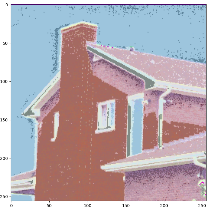
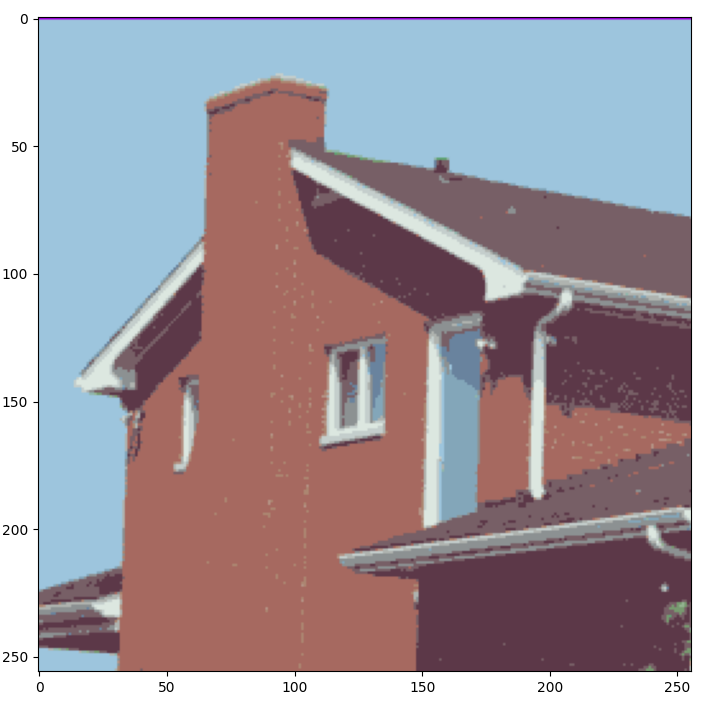
결과사진
 |
 |
| 원본 | 구현한 mean shift |
 |
 |
| 원본 | 구현한 mean shift |
mean shift의 세그멘테이션(segmentation)이 색감별로 잘 적용됨을 확인하였습니다. k means에 비해서 성능이 우수하지만 모든 데이터에 대해서 수렴점을 구하는 과정과 그 수렴점을 군집화하는 과정에서 시간이 많이 소요된다는 단점이 있었습니다.
이제 opencv의 라이브러리를 사용한 결과와 비교해 보겠습니다.
Code(라이브러리)
import numpy as np
import cv2 as cv
from sklearn.cluster import MeanShift, estimate_bandwidth
from matplotlib import pyplot as plt
imageFile = '../lena.bmp'
img1 = cv2.imread(imageFile, cv2.IMREAD_COLOR)
img1 = cv2.cvtColor(img1, cv2.COLOR_BGR2RGB)
img1 = cv2.resize(img1,dsize=(256, 256))
# flatten the image
flat_image = img1.reshape((-1,3))
flat_image = np.float32(flat_image)
# meanshift
bandwidth = estimate_bandwidth(flat_image, quantile=.06, n_samples=3000)
ms = MeanShift(bandwidth, max_iter=800, bin_seeding=True)
ms.fit(flat_image)
labeled=ms.labels_
# get number of segments
segments = np.unique(labeled)
print('Number of segments: ', segments.shape[0])
# get the average color of each segment
total = np.zeros((segments.shape[0], 3), dtype=float)
count = np.zeros(total.shape, dtype=float)
for i, label in enumerate(labeled):
total[label] = total[label] + flat_image[i]
count[label] += 1
avg = total/count
avg = np.uint8(avg)
# cast the labeled image into the corresponding average color
res = avg[labeled]
result = res.reshape((img1.shape))
plt.subplot(1,2,1)
plt.imshow(img1, vmin=0, vmax=255)
plt.subplot(1,2,2)
plt.imshow(result, vmin=0, vmax=255)
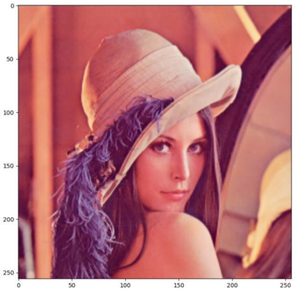
plt.show()결과사진
 |
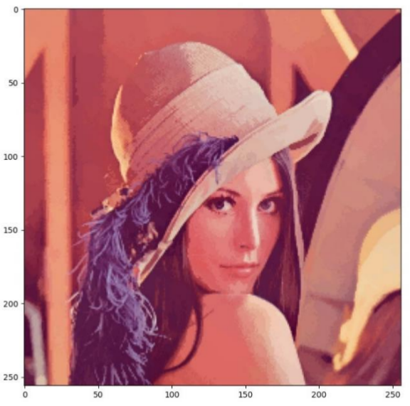 |
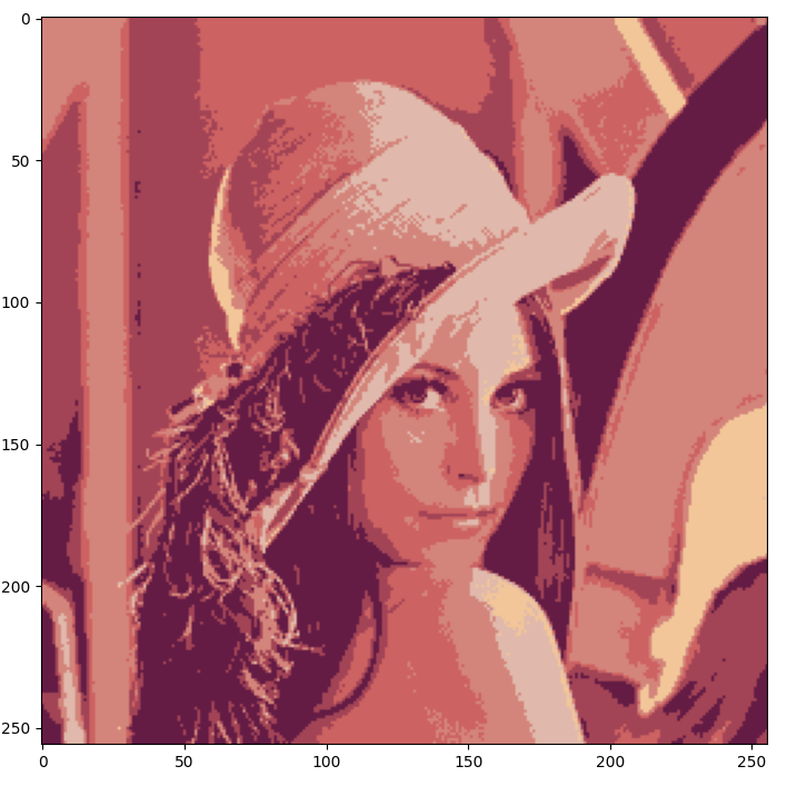
| 라이브러리 | 구현한 mean shift |
 |
 |
| 라이브러리 | 구현한 mean shift |
직접 구현할때는 좌표정보도 rgb값에 추가하여 좌표와 rgb값에 대한 관련성이 높아졌기 때문에 라이브러리보다 더 선명해 보입니다. 이렇게 mean shift를 직접 구현하는데 성공했습니다.
하지만 라이브러리는 10초안에 동작이 된 반면 직접구현한 코드를 실행할때는 2~3분정도 걸렸습니다. 이 부분은 쓰레드 추가와 군집화 알고리즘 개선으로 더 빠르게 처리할수 있다고 생각합니다.
정확한 비교를 위해 이번에는 라이브러리와 같은 조건으로 좌표값을 포함시키지 않고 구현하여 비교해 보겠습니다.
Code(only rgb)
def mean_shift(data, h1):
    w, h, c = data.shape
    data = np.copy(data)
    data = data.reshape(w*h,c)

    v = [] # v is convergence point list
    t = 0

    for i in range(w*h):

            t += 1
            print( (t / (w*h))  * 100) # time(percent)

            y_t = data[i]
            m_s = np.zeros((3))


            while True:
                g = g_k(data, y_t, h1) # g is weights
                g = np.vstack((g,g,g)) # to multiply the same weight
                g = g.T # to make (w*h,3) shape
                deno = np.sum(g) # only sum of weights
                m_s =  np.sum((data - y_t) * g) # m_s is direction vector

                m_s = m_s / deno  # normalization
                temp = np.copy(y_t)
                y_t = y_t + m_s

                if dist(y_t, temp) < 1:

                    v.append(y_t) # append convergence points
                    # print(y_t)
                    break

    label = 0 # num of group
    index_list = [] # to save the index of data

    for i in range(w*h):

        if len(v[i]) == 4: # if len is 4, it is already grouped (length condition).
            continue

        sum = np.copy(v[i]) # v[i] is standard
        count = 1 # to count that how many data belong to that label
        index_list.append(i) # starting from standard

        for j in range(i+1, w*h): # before i, it already had done

            if len(v[j]) == 4: # if len is 4, it is already grouped.
                continue

            if dist(v[i], v[j]) < h1: # if convergence points' distance is less than threshold, suppose that convergence points are same
                    count += 1
                    sum += v[j]
                    v[j] = np.append(v[j],[label]) # to make length condition
                    index_list.append(j) # append that index

        v[i] = np.append(v[i],[label])
        new_value = sum / count # to renew the value of the same convergence point

        for index in index_list:
            data[index] = new_value # data of the same convergence points have the same value (clustering)

        index_list = [] # to empty the index list for the next step
        label += 1 # to increase the num of group for the next step


    print(label)
    return data.reshape(w,h,c)
결과 사진
 |
 |
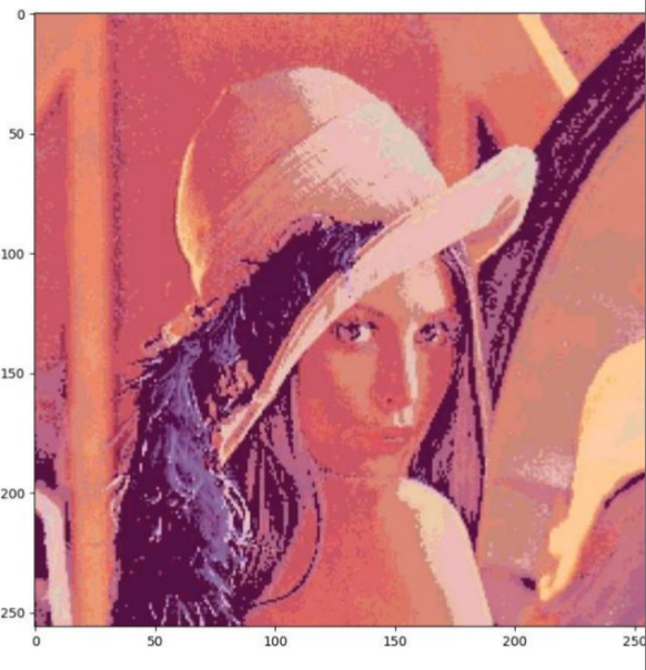
| 구현한 mean shift(rgb) | 라이브러리 |
 |
 |
| 구현한 mean shift(rgb) | 라이브러리 |
색감이 과도하게 밝아진 부분을 제외하면 segmentation은 된것으로 보이나 라이브러리가 성능과 소요시간 면에서 더 우수했습니다.
따라서 직접 구현할때는 앞의 것과 같이 좌표정보도 추가하여 색감과 세그멘테이션에서 보다 정밀하게 구현해야 될것 같습니다.
감사합니다.
'컴퓨터 비전 > 실습' 카테고리의 다른 글
| prewitt, sobel, canny 구현(python) (0) | 2023.02.10 |
|---|---|
| kmeans 직접 구현하기(python) (1) | 2023.01.25 |
| SIFT 직접 구현하기(python) (0) | 2023.01.25 |
| Bilateral Filter 직접 구현하기(python) (0) | 2023.01.18 |


