Bilateral Filter란
이번 포스팅에서는 가우시안 노이즈가 낀 사진을 필터링해주는 Bilateral Filter를 opencv를 사용하지 않고
python으로 직접 구현해 보는것 위주로 다루겠습니다.
Bilateral Filter는 기존 Gaussian Filter와는 다르게 단순히 가우시안 분포(거리에 따라 가중치가 작아짐)로
사진을 복원하는것이 아니라 현재 관심있는 구역의 상태에 따라 동적으로 반영하여 계속 달라지는 필터로 사진을 복원합니다.
예를 들어 원본이 256 * 256 Gray 사진이라면 Gaussian Filter는 Filter가 딱 한개면 되는것에 비해 Bilateral Filter는 무려 약 65536개 만큼 필터를 개별 맞춤 제작해주어야 합니다. 그렇기 때문에 시간이 오래 걸리는데요. 하지만 엣지에서 효과가 Gaussian Filter보다 더 선명하여 단점을 보안한 필터라고 할수 있겠습니다. 코드와 주석을 보시겠습니다.
Code
import cv2
from matplotlib.style import library
import numpy as np
import math
from matplotlib import pyplot as plt
from copy import deepcopy
import random
def G_noise(img, s):
m, n = img.shape
noise = np.random.normal(0, s**2, m * n)
noise = noise.reshape(m, n) # make Gaussian noise ( m * n )
return noise
def Psnr(img1, img2):
m, n = img1.shape
mse = 0
for i in range(m):
for j in range(n):
mse = mse + ((img1[i][j] - img2[i][j]) ** 2.0) # sum of square errors
mse = mse / (m * n) # definition of mean square error
return 20 * math.log10(255 / math.sqrt(mse)) # scaling mse to log scale
def G_filter(k, sigma, v):
assert k % 2 == 1, 'kernel_size must be odd' # filter must be odd_size
n = int((k - 1) / 2) # number to get range of filter
l = []
for i in range(-1 * n, n + 1):
for j in range(-1 * n, n + 1):
c = -1 * ( ( i**2 + j**2 ) / (2 * sigma**2) )
# definition of Gaussian filter
l.append(c)
gaussian = np.exp(l).reshape(-1, k) # take exponential
sum = gaussian.sum() # normalization factor
if v == 1:
return gaussian / sum # version #1
if v == 2:
return gaussian # version #2
def padding(img, n):
x, y = img.shape # original image size
padding_img = np.zeros((x+2*n, y+2*n)) # consider up,down,left,right
padding_img[n:x+n, n:y+n] = img # zero padding
return padding_img
def conv(img, filter):
k = len(filter) # kernel size
n = int((k - 1) / 2) # padding number
x, y = img.shape # original image size
a = padding(img, n)
for i in range(n, x+n):
for j in range(n, y+n):
a[i][j] = np.multiply(a[i-n:i+n+1, j-n:j+n+1], filter).sum() # convolution operation
return a[n:x+n, n:y+n] # return result image ,except the padding part
def Bi_filtered(img, k, sigma_s, sigma_r):
n = int((k - 1) / 2) # padding number
x, y = img.shape
G = G_filter(k, sigma_s, 2) # get Gaussian filter
a = padding(img, n) # padding
for i in range(n, x+n):
for j in range(n, y+n):
b = Bi(a, k, sigma_r, i, j) # get Bilateral filter at present position
filter = np.multiply(G, b) # multiply Gaussian and Bilateral
filter = filter / filter.sum() # normalization
a[i][j] = np.multiply(a[i-n:i+n+1, j-n:j+n+1], filter).sum() # convolution operation
return a[n:x+n, n:y+n]
def Bi(img, k, sigma_r, x, y):
n = int((k - 1) / 2) # number to get range of filter
l = []
for i in range(-1 * n, n + 1):
for j in range(-1 * n, n + 1):
c = -1 * ( ((img[x][y] - img[x+i][y+j])**2) / (2 * (sigma_r)**2) )
# definition of Bilateral
l.append(c)
bilateral = np.exp(l).reshape(-1, k)
return bilateral
def conv(img, filter):
k = len(filter) # kernel size
n = int((k - 1) / 2) # padding number
x, y = img.shape # original image size
a = padding(img, n)
for i in range(n, x+n):
for j in range(n, y+n):
a[i][j] = np.multiply(a[i-n:i+n+1, j-n:j+n+1], filter).sum() # convolution operation
return a[n:x+n, n:y+n] # return result image ,except the padding part
imageFile = '/home/lks9909/image_project1/lena.bmp'
img1 = cv2.imread(imageFile, 0)
noise = G_noise(img1, 5)
img2 = img1 + noise
img3 = conv(img2, G_filter(7,5,1))
img4 = Bi_filtered(img2,7,50,50)
plt.subplot(2,2,1)
plt.imshow(img1, vmin=0, vmax=255, cmap='gray')
plt.subplot(2,2,2)
plt.imshow(img2, vmin=0, vmax=255, cmap='gray')
plt.subplot(2,2,3)
plt.imshow(img3, vmin=0, vmax=255, cmap='gray')
plt.subplot(2,2,4)
plt.imshow(img4, vmin=0, vmax=255, cmap='gray')
plt.show()
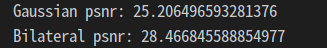
print('Gaussian psnr:', Psnr(img1,img3))
print('Bilateral psnr:', Psnr(img1,img4))결과 비교
 |
|
| 원본 | 원본 + Gaussian Noise |
 |
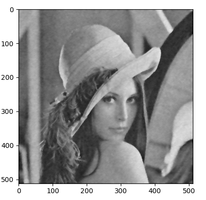 |
| Gaussian Filter 적용 | Bilateral Filter 적용 |
Gaussian Filter는 노이즈가 줄어들긴 했으나 원본에서 블러(blur)가 많이된 것에 비해
Bilateral Filter는 노이즈 제거와 엣지부분에서 선명함을 확인할수 있습니다.
역시 PSNR(최대 신호 대 잡음비)도 더 높음을 확인할수 있습니다.
감사합니다.
'컴퓨터 비전 > 실습' 카테고리의 다른 글
| prewitt, sobel, canny 구현(python) (0) | 2023.02.10 |
|---|---|
| mean shift 직접 구현하기(python) (0) | 2023.01.31 |
| kmeans 직접 구현하기(python) (1) | 2023.01.25 |
| SIFT 직접 구현하기(python) (0) | 2023.01.25 |


